The California Racial Justice Act & San Diego PD RIPA Data

Sreetama Chowdhury

Abstract

Approved in 2020, the California Racial Justice Act allows defendants to appeal for a retrial of their case or an adjustment of the charges or sentencing leveled at them if they can statistically prove that there was racial bias at play. The bill doesn’t actually specify the kind of statistical proof a judge would require, though, so this project is a preliminary search to start to find out what kinds of aspects of criminal justice data might be useful to those invoking the CRJA. To that end, this project used pandas to analyze a dataset of San Diego city traffic stop data collected under RIPA, the Racial and Identity Profiling Act of 2015. It involved preliminary demographic analysis of various aspects of the stop data, outcome testing in the form of variations of the Veil of Darkness test, and a brief investigation into the phenomenon of multiple charges being pressed after the same stop. Analysis showed, however, that there is as of yet no statistically significant evidence of racial bias being involved as a factor of these stops.

Introduction
Methods
Results
Discussion
Sources + Adjacent Data

Introduction

The California Racial Justice Act (AB-2542), approved by the governor in September 2020, is legislation that intends to combat racial bias and disparities in the criminal justice system by offering defendants a chance to contest their cases. The CRJA is usable on multiple levels — checking racial bias both in and out of courtrooms — as it addresses within-court instances of bias as well as racially charged disparities in sentencing, charges, and convictions. If the defendant invoking the CRJA can provide proof of discrimination occurring, a new trial will be set up for the case or the charges or sentence may be adjusted, depending on how far along the court case is.

It’s key legislation in that it not only takes into account intentional bias directed at the defendant (by any other key figure in the courtroom processes) but also racially coded language or interactions. The aspect of the CRJA that this project specifically has focused on is racial disparities in charges. The evidence needed for proof of discrimination in court (when it comes to racial bias in charges) is differences due to race, national origin, or ethnicity in charges on a county-wide basis.

The goal of this project was originally to synthesize a database of information (via extensive data collection, organization, and cleaning) that searches for evidence of racial discrimination, bias, or disparities in terms of individuals stopped by the police and what charges they faced as a result. It ended up focusing on a relatively narrow dataset, using pandas to explore and analyze specifically traffic stop data collected by the San Diego Police Department as part of the Racial and Identity Profiling Act of 2015.

Methods

The actual code used to break down & perform various tests — including outcome testing (in the form of several Veil of Darkness tests) and analysis of stacked charges — on the RIPA stop data.

All data used can be found & downloaded here and on linked pages.

Code

#import + consolidate San Diego RIPA data into one massive df (result_df)

Code

import pandas as pd   
import missingno as msno
import matplotlib.pyplot as plt
import seaborn as sns
import datetime
from datetime import date

from loadRIPA import *
df = loadRIPA()
df['year-month'] = pd.to_datetime(df.date_stop, format='%Y-%m-%d').dt.strftime("%Y-%m")

PART 1: PRELIMINARY DATA BREAKDOWNS & ANALYSIS

Code

#missingno package allows for visualization of missing data within result_df

Code

msno.bar(df)

<AxesSubplot:>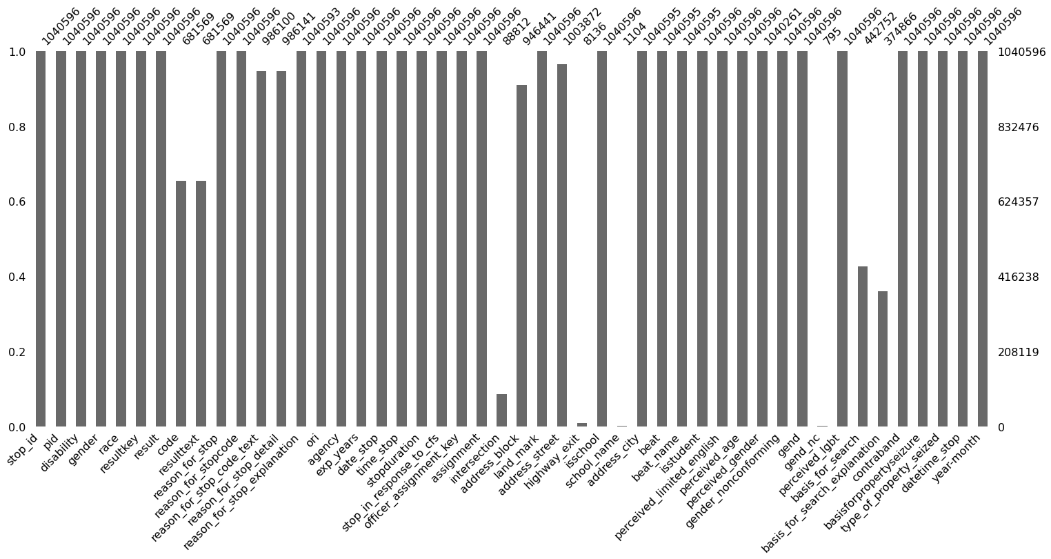

Code

#group the stop data by race + calculate proportions + graph
#to visualize the racial breakdown of the stop data overall

Code

stops_racial_breakdown_df = df.groupby('race', as_index=False).size()
stops_racial_breakdown_df['proportion'] = stops_racial_breakdown_df['size']/stops_racial_breakdown_df['size'].sum()
stops_racial_breakdown_df

	race	size	proportion
0	Asian	47733	0.045871
1	Black/African American	216436	0.207992
2	Hispanic/Latino/a	307737	0.295731
3	Middle Eastern or South Asian	26156	0.025136
4	Native American	2684	0.002579
5	Pacific Islander	10004	0.009614
6	White	429846	0.413077

Code

plt.rcParams['figure.figsize'] = (10, 5)
stops_racial_breakdown_df.plot.barh(x="race", y=["proportion"])
plt.show()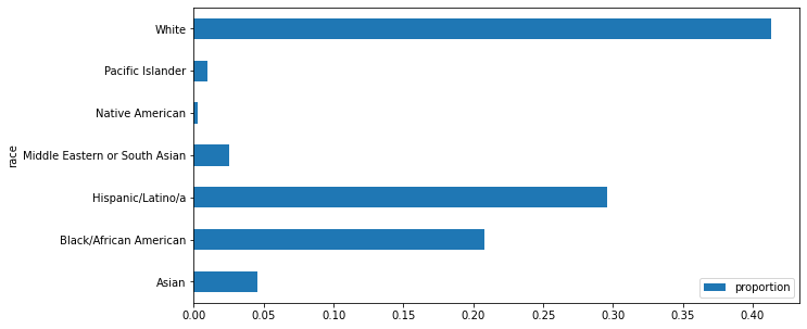

Code

#group stop data by the reason for the stop to calculate + visualize proportions (each reason vs stops overall)

Code

stop_by_reason_df = df.groupby(['reason_for_stop'], as_index=False).size()
stop_by_reason_df['proportion'] = stop_by_reason_df['size']/stop_by_reason_df['size'].sum()
stop_by_reason_df

	reason_for_stop	size	proportion
0	Consensual Encounter resulting in a search	11155	0.010720
1	Determine whether the student violated school ...	78	0.000075
2	Investigation to determine whether the person ...	10608	0.010194
3	Knowledge of outstanding arrest warrant/wanted...	17144	0.016475
4	Known to be on Parole / Probation / PRCS / Man...	15470	0.014866
5	Possible conduct warranting discipline under E...	40	0.000038
6	Reasonable Suspicion	563478	0.541495
7	Traffic Violation	422623	0.406136

Code

stop_by_reason_df.plot.barh(x="reason_for_stop", y=["proportion"])
plt.show()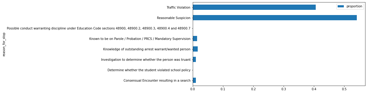

Code

#calculate the racial breakdown (amount & proportion) per each reason for the stop

Code

reason_racial_breakdown_df = df.groupby(['reason_for_stop', 'race'], as_index=False).size()

Code

c_ent = reason_racial_breakdown_df.loc[reason_racial_breakdown_df['reason_for_stop'] == 
                                       'Consensual Encounter resulting in a search' , 'size'].sum()
student = reason_racial_breakdown_df.loc[reason_racial_breakdown_df['reason_for_stop'] == 
                                       'Determine whether the student violated school policy' , 'size'].sum()
truant = reason_racial_breakdown_df.loc[reason_racial_breakdown_df['reason_for_stop'] == 
                                       'Investigation to determine whether the person was truant' , 'size'].sum()
warrant = reason_racial_breakdown_df.loc[reason_racial_breakdown_df['reason_for_stop'] == 
                                       'Knowledge of outstanding arrest warrant/wanted person' , 'size'].sum()
parole = reason_racial_breakdown_df.loc[reason_racial_breakdown_df['reason_for_stop'] == 
                                       'Known to be on Parole / Probation / PRCS / Mandatory Supervision' , 'size'].sum()
conduct = reason_racial_breakdown_df.loc[reason_racial_breakdown_df['reason_for_stop'] == 
                                       'Possible conduct warranting discipline under Education Code sections 48900, 48900.2, 48900.3, 48900.4 and 48900.7' , 'size'].sum()
suspicion = reason_racial_breakdown_df.loc[reason_racial_breakdown_df['reason_for_stop'] == 
                                       'Reasonable Suspicion' , 'size'].sum()
traffic = reason_racial_breakdown_df.loc[reason_racial_breakdown_df['reason_for_stop'] == 
                                       'Traffic Violation' , 'size'].sum()

Code

reason_racial_breakdown_df.loc[reason_racial_breakdown_df.reason_for_stop == 
                              "Consensual Encounter resulting in a search", "total per reason"] = c_ent
reason_racial_breakdown_df.loc[reason_racial_breakdown_df.reason_for_stop == 
                              "Determine whether the student violated school policy", "total per reason"] = student
reason_racial_breakdown_df.loc[reason_racial_breakdown_df.reason_for_stop == 
                              "Investigation to determine whether the person was truant", "total per reason"] = truant
reason_racial_breakdown_df.loc[reason_racial_breakdown_df.reason_for_stop == 
                              "Knowledge of outstanding arrest warrant/wanted person", "total per reason"] = warrant
reason_racial_breakdown_df.loc[reason_racial_breakdown_df.reason_for_stop == 
                              "Known to be on Parole / Probation / PRCS / Mandatory Supervision", "total per reason"] = parole
reason_racial_breakdown_df.loc[reason_racial_breakdown_df.reason_for_stop == 
                              "Possible conduct warranting discipline under Education Code sections 48900, 48900.2, 48900.3, 48900.4 and 48900.7", "total per reason"] = conduct
reason_racial_breakdown_df.loc[reason_racial_breakdown_df.reason_for_stop == 
                              "Reasonable Suspicion", "total per reason"] = suspicion
reason_racial_breakdown_df.loc[reason_racial_breakdown_df.reason_for_stop == 
                              "Traffic Violation", "total per reason"] = traffic

Code

reason_racial_breakdown_df['racial proportion per reason'] = reason_racial_breakdown_df['size']/reason_racial_breakdown_df['total per reason']
reason_racial_breakdown_df.head(7)

	reason_for_stop	race	size	total per reason	racial proportion per reason
0	Consensual Encounter resulting in a search	Asian	393	11155.0	0.035231
1	Consensual Encounter resulting in a search	Black/African American	2233	11155.0	0.200179
2	Consensual Encounter resulting in a search	Hispanic/Latino/a	3273	11155.0	0.293411
3	Consensual Encounter resulting in a search	Middle Eastern or South Asian	169	11155.0	0.015150
4	Consensual Encounter resulting in a search	Native American	56	11155.0	0.005020
5	Consensual Encounter resulting in a search	Pacific Islander	104	11155.0	0.009323
6	Consensual Encounter resulting in a search	White	4927	11155.0	0.441685

Code

#pivot the racial breadown by reason data so that it's easier to visualize 
#visualize in stacked bar chart form

Code

pivoted_df = reason_racial_breakdown_df.pivot(index='reason_for_stop', columns='race', values='size')
pivoted_df

race	Asian	Black/African American	Hispanic/Latino/a	Middle Eastern or South Asian	Native American	Pacific Islander	White
reason_for_stop
Consensual Encounter resulting in a search	252.0	1317.0	2231.0	89.0	30.0	78.0	2777.0
Determine whether the student violated school policy	1.0	4.0	13.0	2.0	NaN	NaN	11.0
Investigation to determine whether the person was truant	346.0	1770.0	2008.0	139.0	27.0	76.0	3241.0
Knowledge of outstanding arrest warrant/wanted person	208.0	1486.0	1619.0	56.0	21.0	53.0	1936.0
Known to be on Parole / Probation / PRCS / Mandatory Supervision	195.0	1757.0	2355.0	58.0	21.0	58.0	2411.0
Possible conduct warranting discipline under Education Code sections 48900, 48900.2, 48900.3, 48900.4 and 48900.7	1.0	NaN	3.0	NaN	NaN	NaN	3.0
Reasonable Suspicion	8518.0	65941.0	73873.0	4577.0	980.0	2351.0	134456.0
Traffic Violation	17408.0	38162.0	79947.0	10326.0	339.0	2354.0	86002.0

Code

pivoted_df.plot.barh(stacked=True)
plt.show()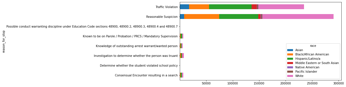

Code

#group data by reason and then result + calculate racial breakdown for each reason/result combination

Code

stop_data_df = pd.merge(race_df, stop_reason_df, how="outer", on=["stop_id","pid"])
stop_data_df = pd.merge(stop_data_df, stop_result_df, how="outer", on=["stop_id","pid"])
result_racial_breakdown_df = stop_data_df.groupby(['reason_for_stop','result', 'race'], as_index=False).size()
result_racial_breakdown_df

	reason_for_stop	result	race	size
0	Consensual Encounter resulting in a search	Citation for infraction	Asian	7
1	Consensual Encounter resulting in a search	Citation for infraction	Black/African American	32
2	Consensual Encounter resulting in a search	Citation for infraction	Hispanic/Latino/a	80
3	Consensual Encounter resulting in a search	Citation for infraction	Middle Eastern or South Asian	8
4	Consensual Encounter resulting in a search	Citation for infraction	Native American	2
...	...	...	...	...
443	Traffic Violation	Warning (verbal or written)	Hispanic/Latino/a	23522
444	Traffic Violation	Warning (verbal or written)	Middle Eastern or South Asian	3156
445	Traffic Violation	Warning (verbal or written)	Native American	121
446	Traffic Violation	Warning (verbal or written)	Pacific Islander	787
447	Traffic Violation	Warning (verbal or written)	White	24407

448 rows × 4 columns

Code

#pivot the racial breakdown by reason/result data so that it's easier to visualize 
#visualize in stacked bar chart form

Code

pivoted_with_reason_result_df = result_racial_breakdown_df.pivot(index=["reason_for_stop", "result"], columns=["race"],values="size")
pivoted_with_reason_result_df = pivoted_with_reason_result_df.div(pivoted_with_reason_result_df.sum(axis=1), axis=0)
pivoted_with_reason_result_df

	race	Asian	Black/African American	Hispanic/Latino/a	Middle Eastern or South Asian	Native American	Pacific Islander	White
reason_for_stop	result
Consensual Encounter resulting in a search	Citation for infraction	0.031390	0.143498	0.358744	0.035874	0.008969	0.031390	0.390135
	Contacted parent/legal guardian or other person responsible for the minor	0.032258	0.225806	0.483871	NaN	NaN	0.032258	0.225806
	Custodial Arrest pursuant to outstanding warrant	0.027732	0.176183	0.337684	0.001631	0.006525	0.004894	0.445351
	Custodial Arrest without warrant	0.023766	0.212066	0.292505	0.005484	0.005484	0.014625	0.446069
	Field interview card completed	0.032003	0.195345	0.364505	0.009559	0.004572	0.010391	0.383624
...	...	...	...	...	...	...	...	...
Traffic Violation	In-field cite and release	0.062540	0.130013	0.333705	0.041534	0.001591	0.010715	0.419902
	No Action	0.059211	0.223636	0.390040	0.030534	0.001737	0.009168	0.285674
	Noncriminal transport or caretaking transport	0.041420	0.165680	0.366864	0.041420	0.005917	0.011834	0.366864
	Psychiatric hold	0.088710	0.201613	0.185484	0.040323	NaN	0.024194	0.459677
	Warning (verbal or written)	0.074127	0.185844	0.334795	0.044920	0.001722	0.011202	0.347391

87 rows × 7 columns

Code

pivoted_with_reason_result_head_df = pivoted_with_reason_result_df.head(5)
pivoted_with_reason_result_head_df.plot.barh(stacked=True)
plt.show()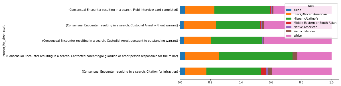

Code

#using seaborn to graph the racial breakdowns of the four most common stop results
#first together, then individually

Code

plt.rcParams['figure.figsize'] = (25, 15)
sns.histplot(data=result_df[result_df['result'].isin(['Citation for infraction', 'Custodial Arrest without warrant', 'Warning (verbal or written)', 'No Action'])], y='race', hue='result', stat='density', multiple='dodge', common_norm=False)

<AxesSubplot:xlabel='Density', ylabel='race'>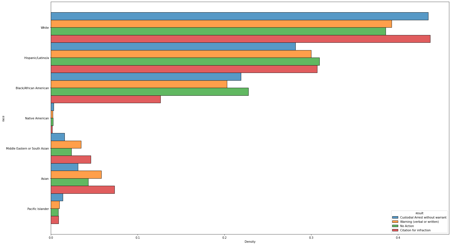

Code

plt.rcParams['figure.figsize'] = (10, 5)
sns.histplot(data=result_df[result_df['result'].isin(['Citation for infraction'])], y='race', hue='result', stat='density', multiple='dodge', common_norm=False)

<AxesSubplot:xlabel='Density', ylabel='race'>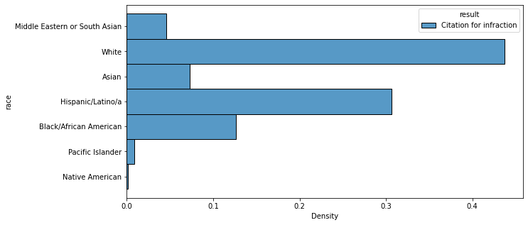

Code

sns.histplot(data=result_df[result_df['result'].isin(['Custodial Arrest without warrant'])], y='race', hue='result', stat='density', multiple='dodge', common_norm=False)

<AxesSubplot:xlabel='Density', ylabel='race'>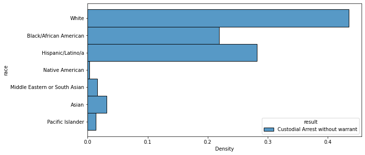

Code

sns.histplot(data=result_df[result_df['result'].isin(['Warning (verbal or written)'])], y='race', hue='result', stat='density', multiple='dodge', common_norm=False)

<AxesSubplot:xlabel='Density', ylabel='race'>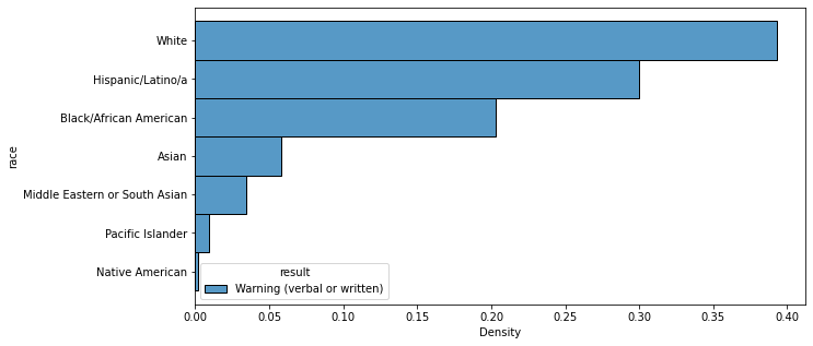

Code

sns.histplot(data=result_df[result_df['result'].isin(['No Action'])], y='race', hue='result', stat='density', multiple='dodge', common_norm=False)

<AxesSubplot:xlabel='Density', ylabel='race'>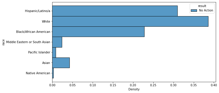

PART 2: VEIL OF DARKNESS TEST(S)

Code

#creating a separate df that includes only the unique identifying features (stop id, PID)
#and the time of each stop (converted to datetime format)

Code

stop_details_df['datetime_stop'] = pd.to_datetime(stop_details_df['date_stop'] + ' ' + stop_details_df['time_stop'])
VOD_df = stop_details_df[['stop_id', 'pid', 'datetime_stop']]
VOD_df = pd.merge(race_df,VOD_df, how="outer", on=["stop_id","pid"])

Code

#creating functions (& corresponding columns)
#that calculate sunrise, sunset, dusk, & dawn times in SD on the day of each stop
#dusk/dawn times are used to calculate whether the stop occurred during the day (ie between dawn/dusk)

Code

from datetime import time
def dateToSunrise(dt):
    if (type(dt) == float):
        return dt #need to fix this
    d = dt.date()
    s = sun(city.observer, date=d, tzinfo=city.timezone)
    return s['sunrise']

def dateToSunset(dt):
    if (type(dt) == float):
        return dt #need to fix this
    d = dt.date()
    s = sun(city.observer, date=d, tzinfo=city.timezone)
    return s['sunset']
    
VOD_df['sunrise'] = VOD_df['datetime_stop'].map(dateToSunrise)
VOD_df['sunset'] = VOD_df['datetime_stop'].map(dateToSunset)

Code

def dateToDawn(dt):
    if (type(dt) == float):
        return dt #need to fix this
    d = dt.date()
    s = sun(city.observer, date=d, tzinfo=city.timezone)
    return s['dawn']

def dateToDusk(dt):
    if (type(dt) == float):
        return dt #need to fix this
    d = dt.date()
    s = sun(city.observer, date=d, tzinfo=city.timezone)
    return s['dusk']
         
def isDaytime(dt):
    if (type(dt) == float):
       return  False # need to fix this 
    if dt.time() > dateToDawn(dt).time() and dt.time() < dateToDusk(dt).time():
        return True
    else:
        return False
    
def isDaytimeFudged(dt):
    if (type(dt) == float):
       return  False # need to fix this 
    dawnFudged =  dateToDawn(dt) + pd.DateOffset(hours=1)
    duskFudged =  dateToDusk(dt) - pd.DateOffset(hours=1)
    if dt.time() > dawnFudged.time() and dt.time() < duskFudged.time():
        return True
    else:
        return False
    
VOD_df['dawn'] = VOD_df['datetime_stop'].map(dateToSunrise)
VOD_df['dusk'] = VOD_df['datetime_stop'].map(dateToSunset)
VOD_df['is_daytime'] = VOD_df['datetime_stop'].map(isDaytime)
VOD_df['is_daytime_fudged'] = VOD_df['datetime_stop'].map(isDaytimeFudged)

Code

earliestDawn = pd.to_datetime('05:11', format = '%H:%M')
latestDawn = pd.to_datetime('06:42', format = '%H:%M')
earliestDusk = pd.to_datetime('17:09', format = '%H:%M')
latestDusk = pd.to_datetime('20:29', format = '%H:%M')

def withinPeriods(dt):
    if (type(dt) == float):
       return  False # need to fix this 
    if dt.time() > earliestDawn.time() and dt.time() < latestDawn.time():
        return False
    elif dt.time() > earliestDusk.time() and dt.time() < latestDusk.time():
        return False
    else:
        return True
    
VOD_df['original_VOD'] = VOD_df['datetime_stop'].map(withinPeriods)

Code

VOD_df

	stop_id	pid	race	datetime_stop	sunrise	sunset	dawn	dusk	is_daytime	is_daytime_fudged	original_VOD
0	2443	1	White	2018-07-01 00:01:37	2018-07-01 05:44:42.442709-07:00	2018-07-01 20:00:13.737456-07:00	2018-07-01 05:44:42.442709-07:00	2018-07-01 20:00:13.737456-07:00	False	False	True
1	2444	1	White	2018-07-01 00:03:34	2018-07-01 05:44:42.442709-07:00	2018-07-01 20:00:13.737456-07:00	2018-07-01 05:44:42.442709-07:00	2018-07-01 20:00:13.737456-07:00	False	False	True
2	2447	1	Hispanic/Latino/a	2018-07-01 00:05:43	2018-07-01 05:44:42.442709-07:00	2018-07-01 20:00:13.737456-07:00	2018-07-01 05:44:42.442709-07:00	2018-07-01 20:00:13.737456-07:00	False	False	True
3	2447	2	Hispanic/Latino/a	2018-07-01 00:05:43	2018-07-01 05:44:42.442709-07:00	2018-07-01 20:00:13.737456-07:00	2018-07-01 05:44:42.442709-07:00	2018-07-01 20:00:13.737456-07:00	False	False	True
4	2448	1	White	2018-07-01 00:19:06	2018-07-01 05:44:42.442709-07:00	2018-07-01 20:00:13.737456-07:00	2018-07-01 05:44:42.442709-07:00	2018-07-01 20:00:13.737456-07:00	False	False	True
...	...	...	...	...	...	...	...	...	...	...	...
535234	478837	2	Hispanic/Latino/a	2021-09-30 17:39:00	2021-09-30 06:42:31.069332-07:00	2021-09-30 18:33:50.427246-07:00	2021-09-30 06:42:31.069332-07:00	2021-09-30 18:33:50.427246-07:00	True	True	False
535235	478845	1	White	2021-09-30 21:00:00	2021-09-30 06:42:31.069332-07:00	2021-09-30 18:33:50.427246-07:00	2021-09-30 06:42:31.069332-07:00	2021-09-30 18:33:50.427246-07:00	False	False	True
535236	478867	1	White	2021-09-30 15:50:00	2021-09-30 06:42:31.069332-07:00	2021-09-30 18:33:50.427246-07:00	2021-09-30 06:42:31.069332-07:00	2021-09-30 18:33:50.427246-07:00	True	True	True
535237	478867	2	White	2021-09-30 15:50:00	2021-09-30 06:42:31.069332-07:00	2021-09-30 18:33:50.427246-07:00	2021-09-30 06:42:31.069332-07:00	2021-09-30 18:33:50.427246-07:00	True	True	True
535238	478934	1	Black/African American	2021-09-30 22:30:00	2021-09-30 06:42:31.069332-07:00	2021-09-30 18:33:50.427246-07:00	2021-09-30 06:42:31.069332-07:00	2021-09-30 18:33:50.427246-07:00	False	False	True

535239 rows × 11 columns

Code

#group all stops by whether they take place during day or night.

Code

sns.histplot(data=VOD_df, y='race', hue='is_daytime', stat='density', multiple='dodge', common_norm=False)

<AxesSubplot:xlabel='Density', ylabel='race'>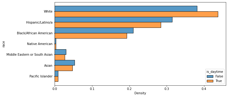

Code

#fudge the values used to calculate whether or not a stop occurred during the day
#by an hour on each end
#to check for any discrepancies or changes when it comes to the early morning or the beginning of night

Code

sns.histplot(data=VOD_df, y='race', hue='is_daytime_fudged', stat='density', multiple='dodge', common_norm=False)

<AxesSubplot:xlabel='Density', ylabel='race'>

Code

#the original VOD test involves removing ambiguity about dusk or dawn
#by counting any stops that occurred between the earliest & latest dusk or dawn times
#as night rather than day
#the two graphs below are visualizations of the breakdown of stops that occurred 
#during the 'day' and during the 'night' (incl. dusk and dawn times)

Code

original_VOD_df = VOD_df[VOD_df['original_VOD'] == True]
sns.histplot(data=original_VOD_df, y='race', hue='is_daytime_fudged', stat='density', multiple='dodge', common_norm=False)

<AxesSubplot:xlabel='Density', ylabel='race'>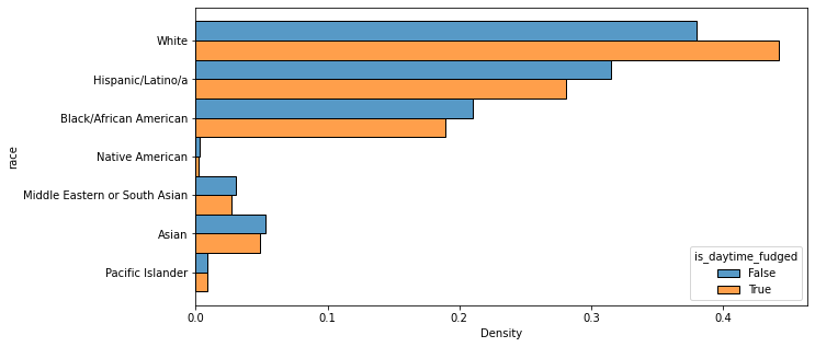

Code

original_VOD_df_2 = VOD_df[VOD_df['original_VOD'] == False] 
sns.histplot(data=original_VOD_df_2, y='race', hue='is_daytime', stat='density', multiple='dodge', common_norm=False)

<AxesSubplot:xlabel='Density', ylabel='race'>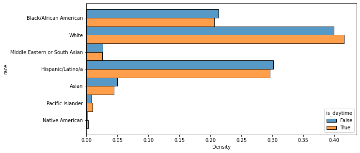

PART 3: MULTIPLE CHARGES

Code

#creating a df of only stop id/pid combinations that have more than one charge (ie, stop result) attached to them

Code

unique_stop_df = stop_data_df.groupby(['stop_id','pid'], as_index=False).size() 
multiple_charges_df = unique_stop_df[unique_stop_df['size'] > 1]
multiple_charges_df

	stop_id	pid	size
7	2453.0	1.0	2
15	2462.0	1.0	2
40	2490.0	1.0	2
50	2505.0	1.0	2
53	2508.0	1.0	2
...	...	...	...
529550	478621.0	1.0	4
529554	478625.0	1.0	2
529573	478642.0	1.0	2
529578	478651.0	1.0	2
529593	478834.0	1.0	2

53742 rows × 3 columns

Code

multiple_charges_df['size'].describe()

count    53742.000000
mean         2.291895
std          0.859710
min          2.000000
25%          2.000000
50%          2.000000
75%          2.000000
max         24.000000
Name: size, dtype: float64

Code

multiple_charges_df['size'].value_counts()

2     44763
3      5017
4      2915
6       478
5       294
8       110
7        40
9        38
12       32
10       31
16       10
15        6
18        3
14        2
24        2
20        1
Name: size, dtype: int64

Code

#visualizing the racial breakdown of people with 2-4 (inclusive) charges
#as those are by far the most common

Code

common_multiple_charges_df = multiple_charges_df[multiple_charges_df['size'] <= 4 ]
temp_df = result_df[['stop_id', 'pid', 'race']]
common_multiple_charges_df = pd.merge(temp_df, common_multiple_charges_df, how="inner", on=["stop_id","pid"])

Code

common_multiple_charges_df = common_multiple_charges_df.drop_duplicates()
sns.histplot(data=common_multiple_charges_df, y='size', hue='race', multiple='dodge', common_norm=False)

<AxesSubplot:xlabel='Count', ylabel='size'>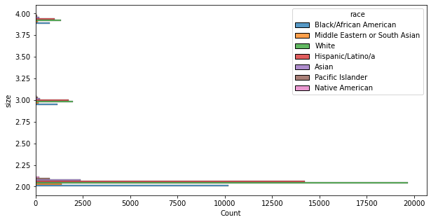

Results

First and foremost, breaking down the racial makeup of the overall RIPA stop data revealed that while the majority of racial categories made up approximately the same proportion of the stop data as they did the overall population of San Diego, the Black/African American community was vastly overrepresented. African Americans, who only account for 6.4% of the population of the city of San Diego, made up almost 20% of the RIPA stop data.

The most common reasons for an individual being stopped were “Reasonable Suspicion” and “Traffic Violation” by far. The vast majority of people stopped for either of these reasons were white, followed by Hispanic/Latinx and then Black/African American. Hispanic/Latinx individuals made up around 25.7% and 34.5%, respectively, of stops for “Reasonable Suspicion” and “Traffic Violation,” while Black/African American individuals made up around 22.9% and 16.5% of the same.

All of these percentages are similar enough to the overall percentages of Hispanic/Latinx and Black/African American people stopped — around 29.5% and 19.9%, respectively, which don’t differ significantly from the percentages of people in these demographics stopped for the two most common reasons. This exploration is therefore inconclusive, as there’s no visible statistical evidence to prove that a disproportionate number of Hispanic/Latinx or Black/African Americans were stopped due to racial bias.

Visualization of the racial breakdown of each possible combination of the reason for the stop and the result of the stop showed similar results. The vast majority of people whose stops involved each reason/result combination were white, followed again by Hispanic/Latinx, followed again by Black/African American, and none of the corresponding percentages were different enough from the overall stop racial percentages to indicate any provable bias. The exceptions in this case were those combinations whose numbers were so small as to be statistically insignificant entirely.

Similarly, when the racial breakdowns of the four most common results of a traffic stop (“Custodial Arrest without warrant,” “Warning (verbal or written),” “No Action,” and “Citation for infraction”) were calculated and graphed, the findings were the same: white majority, followed by Hispanic/Latinx and then Black/African American, with no statistical evidence of racial bias.

The data was also put through the Veil of Darkness test, which involves separating the hours of a given day into categories based on whether they are or are not between dawn and dusk. The logic of the VOD test is that racial bias during police stops (if it exists, that is) should be exaggerated during the daytime because it’s objectively harder for a police officer to identify the race of someone in a car in the dark. Three variations of the test were performed, with one splitting a day into daytime and night as explained above (i.e., between dawn and dusk or not) and the second doing the same except with an hour added to dawn and subtracted from dusk to account for Daylight Savings time. The third dissected the data further by separating out any stops that occurred in the periods between the earliest and latest dawns of the year and the earliest and latest dusks of the year, to avoid any possible ambiguity about when the environment might have been dark.

For every single test variation, though, every racial category other than White had more instances of stops at night than stops during the daytime, which is the exact opposite result than would be expected for proof of racial bias.

The final exploratory step taken involved the racial breakdown of stops that resulted in multiple charges, as (according to lawyer Coleen Cusack) it’s not unheard of for officers to use “stacked charges” as a punitive measure — pressing charges above a certain number mandates an appearance in court, something many defendants have trouble affording to do.

However, the results of this were roughly the same as those of the very first set of data explorations: white people were the majority of instances of stacked charges, and the demographics with the next-highest numbers (Hispanic/Latinx and Black/African American, again) didn’t appear in proportions that were significantly different from the percentages of their demographic appearing in the stops overall.

Discussion

The one key aspect of this project that statistically pointed towards bias was the original racial breakdown of the entire collection of stops; as previously mentioned, the African American community was overwhelmingly overrepresented in police stop data when compared to the actual demographics of the city of San Diego. Every other test, however, resulted in a key lack of provable statistical evidence of bias, so this project cannot properly conclude that there was any bias affecting the outcomes of police stops and the resultant charges.

That said, the results of this project are not necessarily generalizable to the entire court system or even to the entire county. The data measured here is San Diego city data, which isn’t representative of the state as a whole or even of San Diego County. It’s also data specific to traffic stops, which are far from the only source of entry into the criminal justice system. Even if any proof of bias was found, it wouldn’t necessarily hold up in a court of law due to the fact that the text of the CRJA requires statistical proof of racial discrimination on a county-wide scale. Ultimately, rather than being a sweeping examination of police data and bias in criminal justice across the state of California as a whole, this project was more of an introductory exploration to see if there’s anything on a smaller scale that might also occur on a larger scale before we investigate larger amounts of data. Patiently working through the same forms of exploration with larger, more general datasets could well lead to statistical windfalls.

The California Racial Justice Act & San Diego PD RIPA Data

Abstract

Table of Contents

Introduction

Methods

Results

Discussion

Sources + Adjacent Data

Introduction

Methods

PART 1: PRELIMINARY DATA BREAKDOWNS & ANALYSIS

PART 2: VEIL OF DARKNESS TEST(S)

PART 3: MULTIPLE CHARGES

Results

Discussion

Sources + Adjacent Data

Sources

Software

Adjacent Data